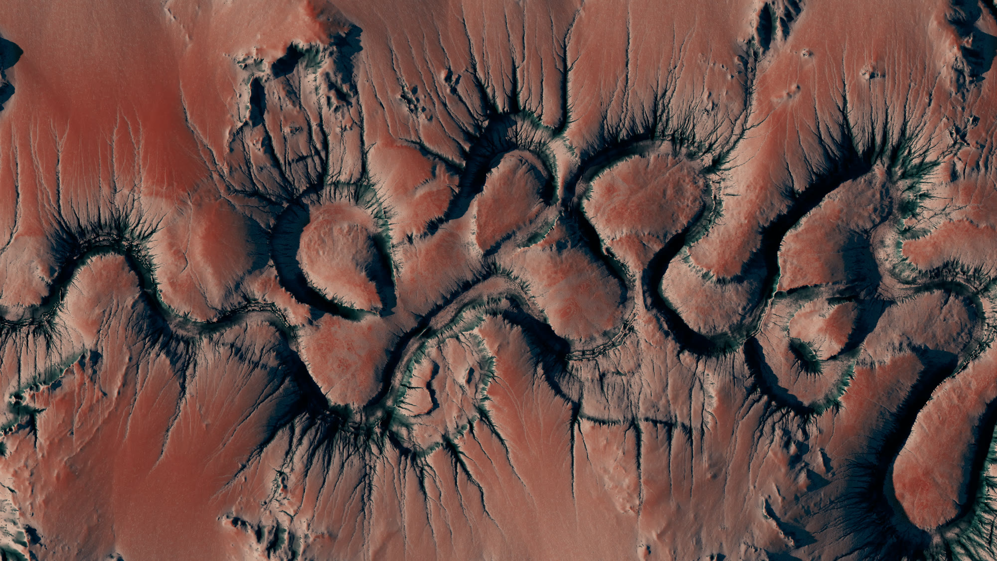
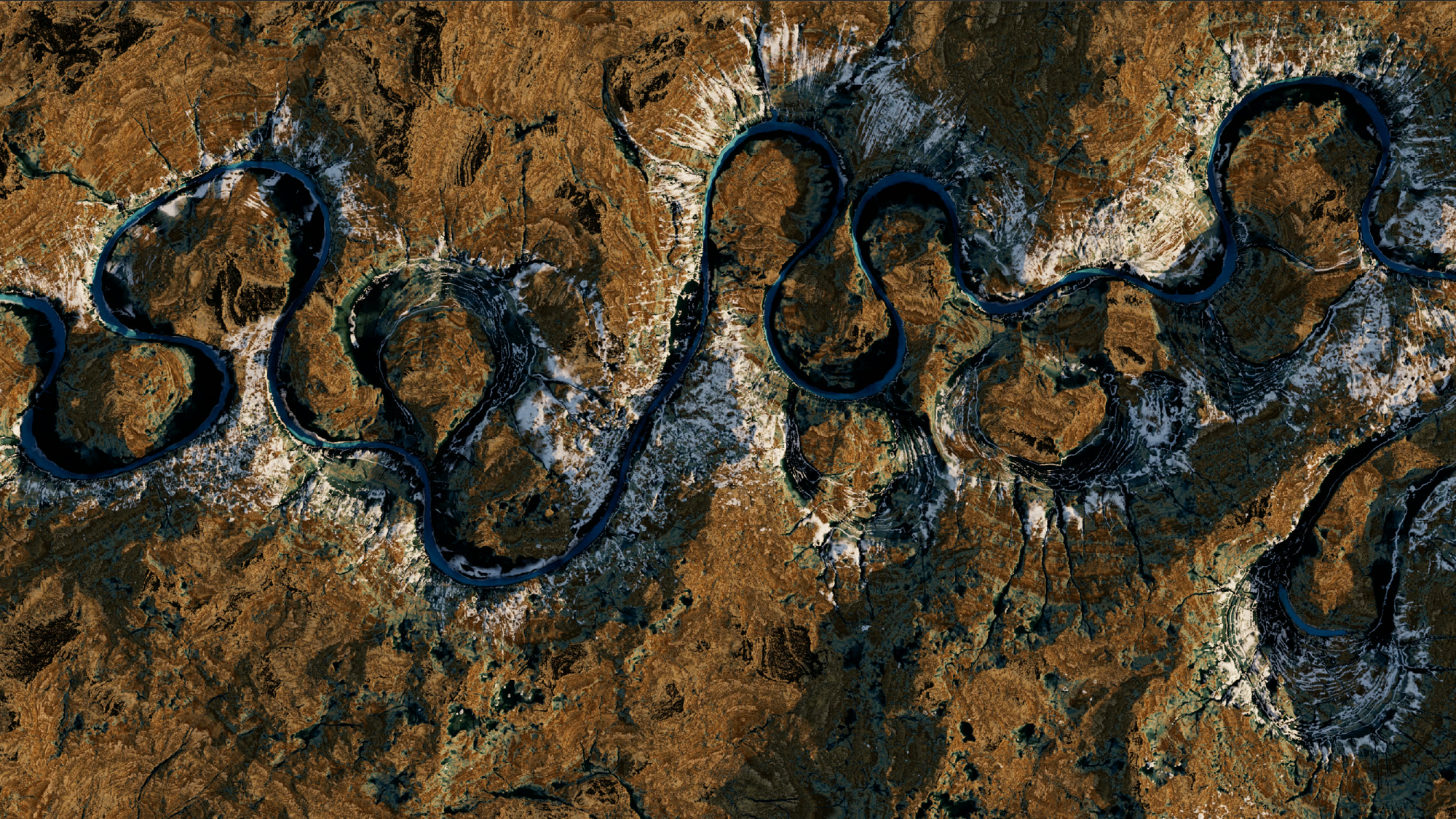
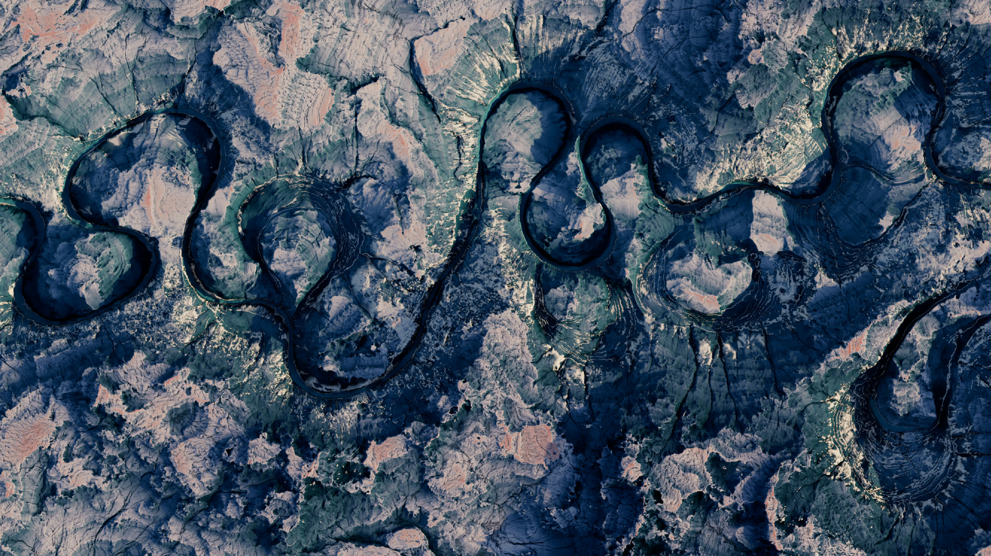
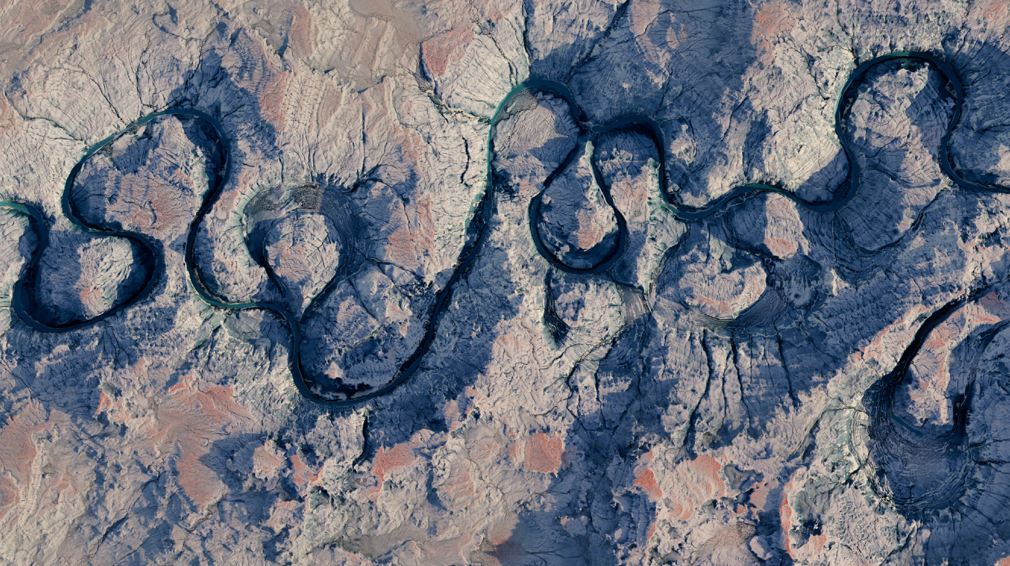
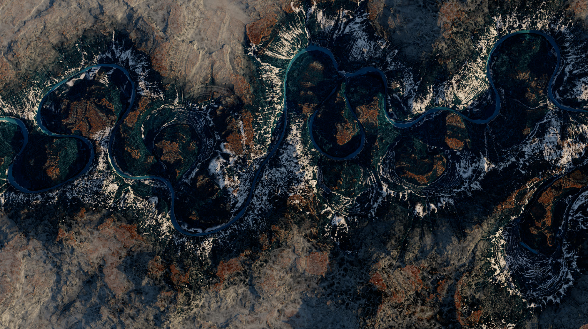
A Houdini simulation in which a single curve develops into a meandering river over many frames. Each frame a curvature signal pushes the channel sideways; oxbow lakes appear when two stretches drift close enough that a shortcut edge bridges the neck and the channel crosses it, leaving the abandoned arc behind. The same step that updates the channel produces the topology change.
Methods
Houdini · Simulation · Geomorphology
1 · intuition
Real rivers bend through a short feedback loop:
Flow erodes the outer bank of a curve, pushing the channel further outward.
Over time the bend grows and the curvature exaggerates.
Two non-adjacent stretches eventually drift close enough that the flow takes a shortcut, cuts the neck, and leaves the abandoned arc behind as an oxbow lake.
The simulation translates that loop into geometry. A curvature signal picks the direction every point on the curve should be pushed, and a small set of topology rules handles the cut-offs at the right moment.
2 · approach
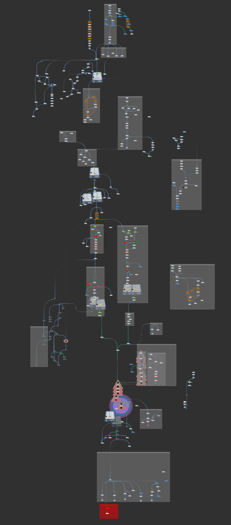
Houdini network — meandering-river solver
Pipeline:
init curve ──► per-frame solver ──► river + accumulated oxbows
Initial curve
A straight line, evenly resampled, with a few layers of noise displacement applied across the middle. The displacement weight tapers to zero at both ends so the endpoints stay anchored from the start. This wobbled line is the seed the solver evolves from.
Each solver step
Compute the offset direction. The signed mean curvature of the current channel is measured and combined with the local tangent into a per-point displacement vector — a lateral push with a small downstream component. The push is again weighted to zero at the endpoints, so the channel only moves in its interior.
Push and reconnect. The displacement is added to each point. Nearby point pairs are then connected with shortcut edges, but only when they sit within a small search radius and their tangents are close to parallel. The parallel-tangent condition keeps the connection step local; without it, distant points across the canvas can also fall within the radius and get wired together.
Re-trace the channel. The channel is re-traced from start to end through the augmented graph. Where a shortcut edge bridges a neck, the trace crosses it instead of following the loop the long way around.
When a shortcut bridges the neck, the channel crosses it — cutting through what was a wider loop.
The bypassed loop, no longer on the channel, becomes the new oxbow.
The same re-tracing step that updates the channel also separates the oxbow from it, so the topology change happens as part of the ordinary update.
Smooth and pin. A few rounds of blur and smooth keep the channel readable. A final pass identifies the channel's two endpoints by neighbour count — a real endpoint has exactly one neighbour — and locks them back to their initial positions. Oxbows are closed loops, so they have no one-neighbour points and stay out of this pass.
Old oxbows accumulate in the output, so a long run shows the river drifting across the canvas with the previous channels visible behind it.
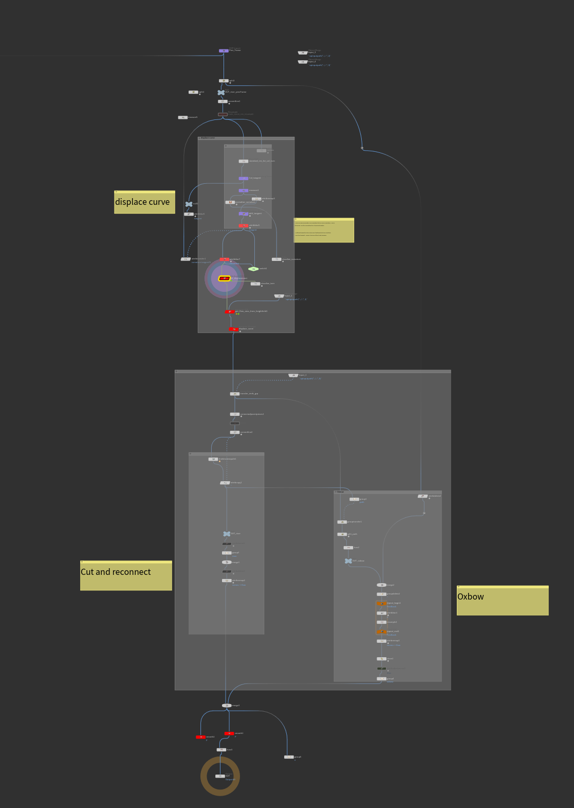
The same network annotated — displace curve, cut & reconnect, oxbow
3 · properties
Long-running stability. The solver has no fixed length. Once balanced, it can keep going for thousands of frames, and the shape continues to mature as it runs.
Topology change inside the update step. Oxbow formation uses the same shortcut-edge plus re-tracing step that produces each new channel, so a separate self-intersection check is unnecessary.
A small set of knobs. Displacement strength, smoothing strength, and the search radius and cone angle for shortcut connection are the main parameters. Together they set how aggressively the river rewrites itself each frame.
4 · side experiment · closed loops
I tried the same approach on a closed curve — a ring-shaped river with no start and no end. Mixed result:
✓ The closed topology is preserved through the solver chain, and the feedback loop still evolves the curve.
✗ The lateral-displacement signal assumes an upstream / downstream direction. On a closed loop it instead pulls the whole ring toward its centroid, so the curve shrinks rather than meandering.
✗ The re-tracing step has nothing to trace between on a closed loop. A ring has no start or end, so there is no channel to re-trace; splitting one ring into two would need a different graph operation.
A working closed-loop version would need three different pieces: an arc-length-integrated upstream curvature signal (a simplified Howard–Knutson), Taubin smoothing in place of plain Laplacian so the ring doesn't contract toward its centroid, and a graph-theoretic ring-splitting routine in place of the start-to-end re-trace. That is a separate project.