← studies·status: in progress·phase 8.6 → 9·last update 2026-04-17
NCA Ecology — emergence under learned rules
Rules → emergence, with AI as part of the rule itself. An open-ended exploration: no target shape is declared up front; what the kernel can become is the question, and the surprises along the branches are the answer.
// 0 · why constraint geometry
A neural cellular automaton is a tiny update rule (≈8K parameters) applied locally to every grid cell, run for many steps, trained end-to-end through the rollout. The interesting design surface is the loss. The kernel learns whatever physics the loss asks it to preserve.
What makes this path different from a Houdini PDE solver is that the loss can target objects an Euler–Lagrange machinery cannot express: trajectory statistics, cross-scale information, learned perceptual losses. SGD reaches them. Closed-form variational physics does not.
What follows reads as a lab notebook. Each card is one direction the constraint geometry was pushed in, kept whether or not it converged. The page is messy on purpose; a tidied-up version would lose the side-trips, and the side-trips are where the surprises live: a trivial solution that turns out visually rich (§ 1.04), a transient window of structure the loss curve never noticed (§ 1.03), an attractor that only appears at one specific resolution (§ 4.03). The pattern that emerges across the cards is the actual finding. The same small loss family produces dunes, mycelium, vertical wires, labyrinths, coffee-oil holes, and tree bark, each at its own bend in the design space.
constraint geometry
────────────────────────────────────────────────────────────────

   classical PDE                    this project
   ──────────────                   ────────────────────
   write the equation               write the constraints
   integrate                        SGD searches a rule
                                    that satisfies them all

   reaches                          reaches
   = equations humans have          = any autodiff-friendly
     written down                     function, including
                                      PDE-unwritable ones:
                                       · trajectory statistics
                                       · cross-scale information
                                       · topological invariants
                                       · learned perceptual losses
§ 1 · early loss design
Texture field
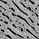
Pre-architectural-conservation runs. Loss-as-physics: pick three terms, watch what the kernel does. Most outputs are dunes and fingerprints; a handful of side-runs find something stranger.
First loss that produced a non-trivial steady state. Three terms: soft mass conservation, multi-scale spatial heterogeneity (encourage structure), anti-stasis (penalise dead frames).
Result: fingerprint/dune at every λ ratio. Sets the ceiling of what residual-ΔM kernels with this loss family can reach. Used as the baseline that every later card compares against.
005 · 2k005 · 5k005 · 10k003 · 3k003 · 5k002006
§ 1.02 · advection_diffusion_020·stable · clean
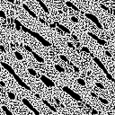
Diagonal fingerprint — naming the channels
Channels are given physical identity (M = mass, V = velocity). The conservation term becomes an advection–diffusion tension pair: linear advection wants to grow structure, quadratic Dirichlet caps it. Small ∇M is advection-dominated, large ∇M is Dirichlet-dominated.
First time the kernel learned a non-trivial physics over named channels. Pattern is cleaner than the dune baseline because the velocity field picks a direction; the diagonal hatching is stable across the entire training window.
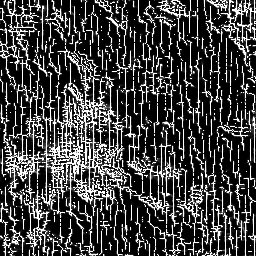
§ 1.03 · conservation_physics_008·transient · interesting in window
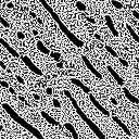
Tents → vertical texture → collapse
Same loss as 1.01 but trained 2× longer (20k steps instead of 10k). What the loss curve hides: the kernel transiently invents two structures before pool collapse erases everything.
Steps 700-3000: triangle/tent structures (early dune-formation phase, never noticed at 10k cutoff). Steps 8400-11200: a different attractor with vertical hatching that conservation_005 never reached. Past step 14000 every loss term decays to zero and the field goes uniform. Pool diversity collapses faster than the rule can find something stable. The interesting visual structure exists only in the window between two failures.
§ 1.04 · dissipative_physics_004·trivial static solution · visually best in this section
Mycelium mesh — degenerate but rich
Adds a radial source/sink injection at every NCA step. After step 1000 the kernel learns a precise static compensation function (delta ≈ −source + sink); conservation and anti-stasis both decay to zero and only heterogeneity is still gradient-active.
Technically a degenerate solution. The kernel doesn't actually do dynamics. But because the source/sink field is spatially non-uniform, the static compensation it learns is also non-uniform, and heterogeneity decorates that scaffold with two visually distinct attractors: bright blob clouds (mode A) and dark mycelium-mesh patches (mode B). Same training, alternating per pool state. The most-photographed run of this phase, even though the rule is doing the wrong thing for the right reasons.
A try at a stronger spatial-heterogeneity term inside the physical-channels architecture. Loss gets eaten by point-like attractors. Mass over-concentrates into bright dots and short radial streaks on a near-empty background; every gradient is shouting in the same direction.
Counted as a failure because the heterogeneity is fake (it's variance from the empty background, not from real structure). Kept here because the radial-dot phase by itself is a useful visual that the rest of the project hasn't reproduced any other way.
Source/sink without the strict-conservation guard from 1.04. The cheapest way to satisfy the loss is to copy the input field back out, and the kernel converges exactly there. A bright disk that traces the radial source.
Mid-training (steps 6000-8000) it briefly explored half-dune patches in the high-flux regions. Those frames are the only thing worth keeping from this run.
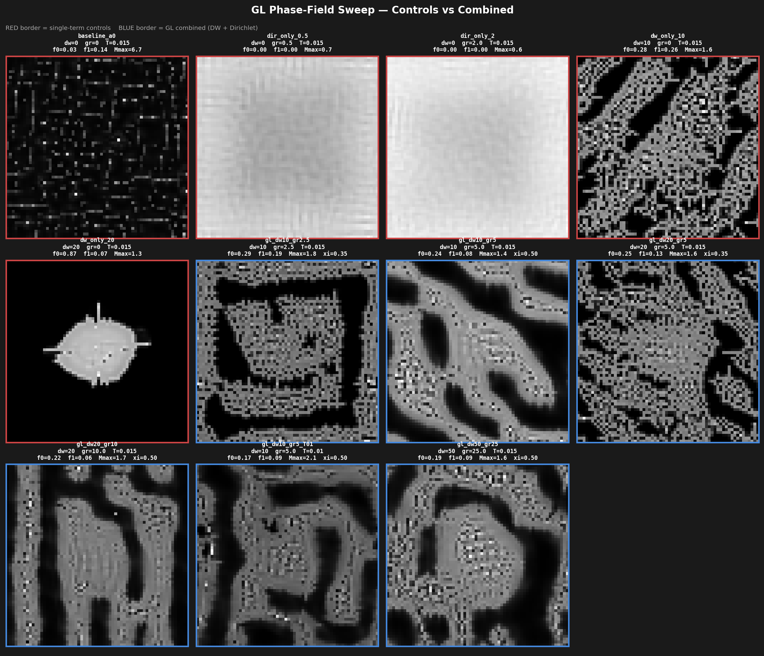
Replace the tension-pair with an explicit Ginzburg-Landau free energy. Buys scale invariance: the same 64² checkpoint runs unchanged at 1024². The visual quality stays mid until the next section adds multi-scale perception.
Different loss family. Replace the tension pair with an explicit free-energy functional and a width-setting Dirichlet term:
F = U(M) − T·H(M) + γ·M²(1−M)² + (κ/2)·‖∇M‖²
The double-well γ-term creates two phases; the Dirichlet κ-term sets the interface width. Sweep over dw / gr / T. Most variants look mid; a few of them (dw=20, gr=10) lock into stable labyrinths with multi-pixel walls. Bonus: the same 64² checkpoint runs unchanged at 1024², because line widths are scale-invariant.
dw20 gr10dw20 gr5dw10 gr5dw50 gr25dw only 10dw only 20dir only 0.5dir only 2
GL phase-field sweep · red = single-term controls, blue = combined
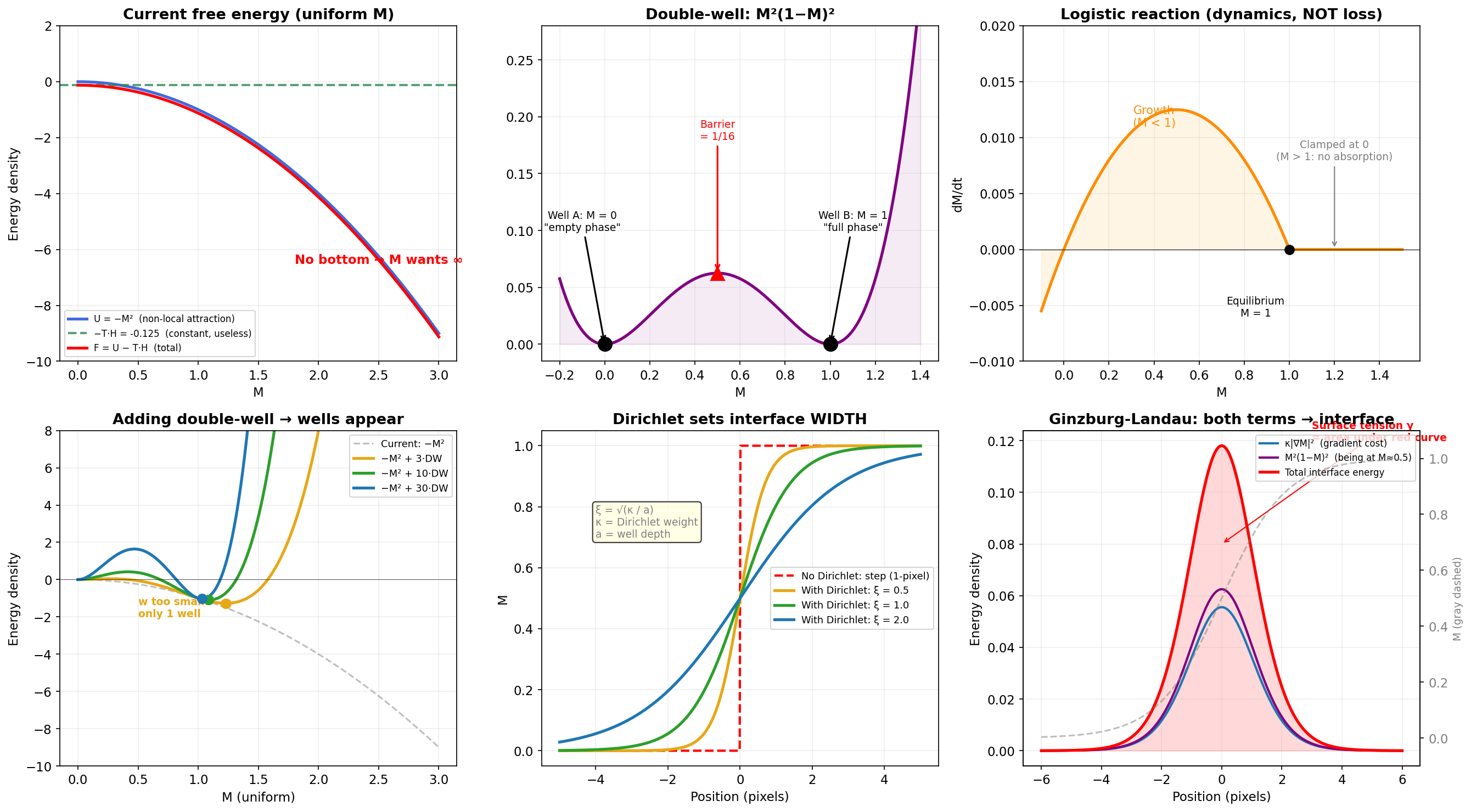
§ 2.02 · energy_landscape_diagnostic·design note
What each loss term does
Six-panel reference plot from when the GL loss was being put together. Top row: the bare free energy, the M²(1−M)² double-well barrier, and the logistic reaction term (which is in the dynamics, not the loss). Bottom row: how adding the double-well term builds wells, how Dirichlet sets the interface width, and the two terms combined giving a finite-width interface energy. Useful as a sidebar; not visually special.
energy-landscape diagnostic · matplotlib
§ 3 · phase 8.6
Multi-scale perception — coffee-oil
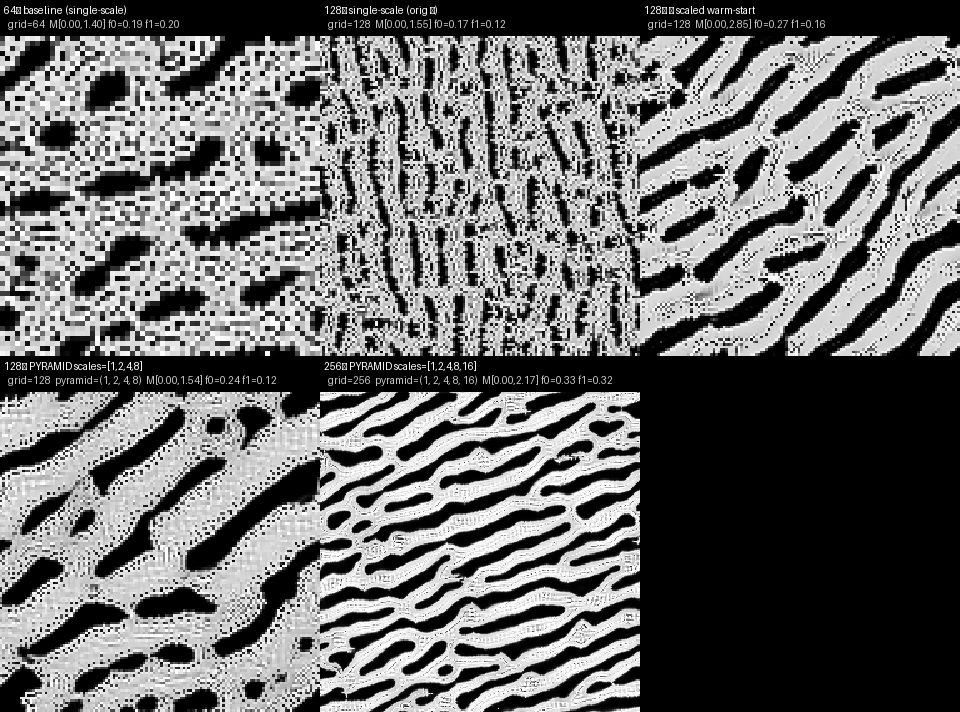
DyNCA-style perception pyramid (DoG at scales 1, 2, 4, 8, 16) applied to the GL loss. Worm width scales with the field. The best-looking attractor in the project came out of this section. Most of the surrounding ablations confirm how narrow the good window is.
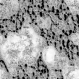
§ 3.01 · phase86_coffee_oil·best attractor of the project
Coffee-oil — multi-scale perception
Add a DyNCA-style perception pyramid: the same DoG kernel applied at scales 1, 2, 4, 8, 16, summed before the MLP. Same loss family as 2.01, same kernel size; the worm width scales from ~10px at 64² baseline to ~30-60px at 256² pyramid.
The phase-separation indicator f₀+f₁ climbs from 0.20 at the single-scale baseline to 0.65 at 256² pyramid. Currently the most cinematic attractor in the project.
pilot 64²g128 pyramidg256 pyramidno-grad (control)low-grad 0.25
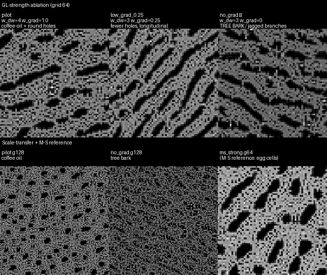
Same 64² pilot but with the gradient term scaled down (0.25× and 0×). The full GL pilot gives round coffee-oil holes. Cutting gradient weight by 4× gives fewer, longitudinal holes. Removing it entirely gives jagged tree-bark fragments. Scale-transferring up to 128² breaks down. The bottom row is the M-S (mean–subtract) reference for comparison, which gives the egg-cell look.
GL-strength ablation · grid 64² + scale-transfer at grid 128²
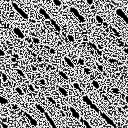
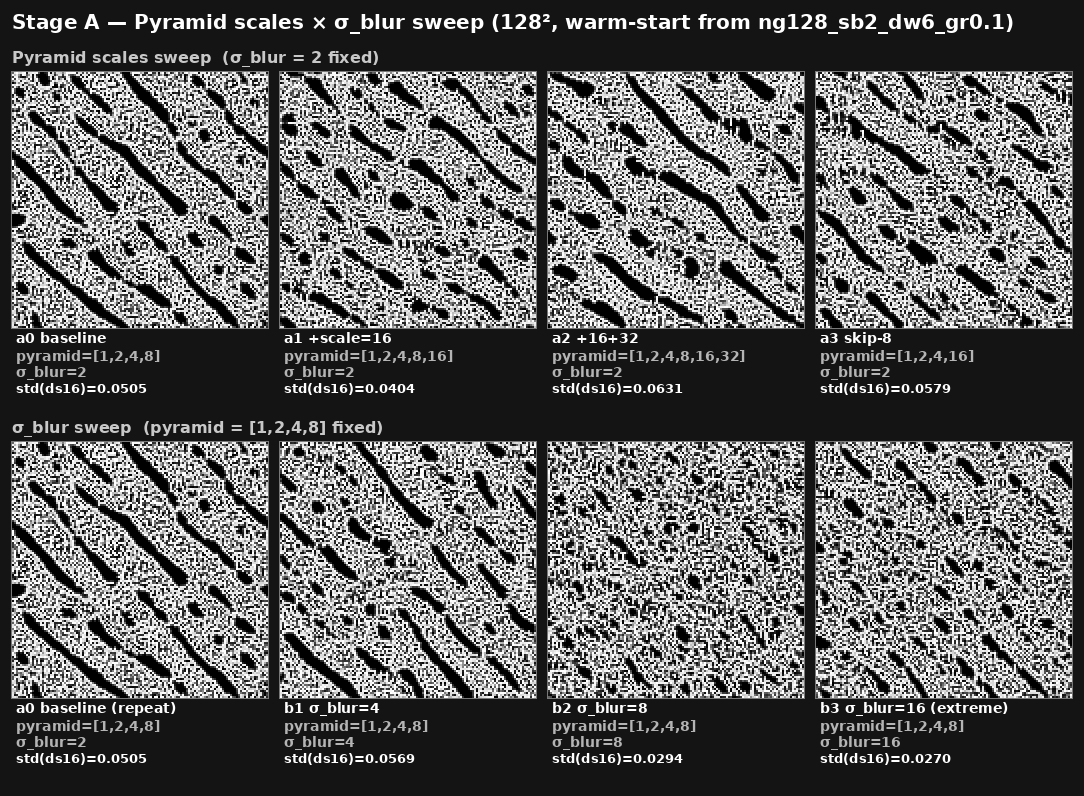
Holding the coffee-oil loss fixed, sweep the perception pyramid scale set and σ_blur. All seven variants land in roughly the same attractor (fine intricate worms), with minor differences in line density. Useful negative result: once the loss is right, the pyramid shape is not very sensitive.
Stage A pyramid scan · warm-start from ng128_sb2_dw6_gr0.1
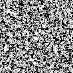
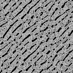
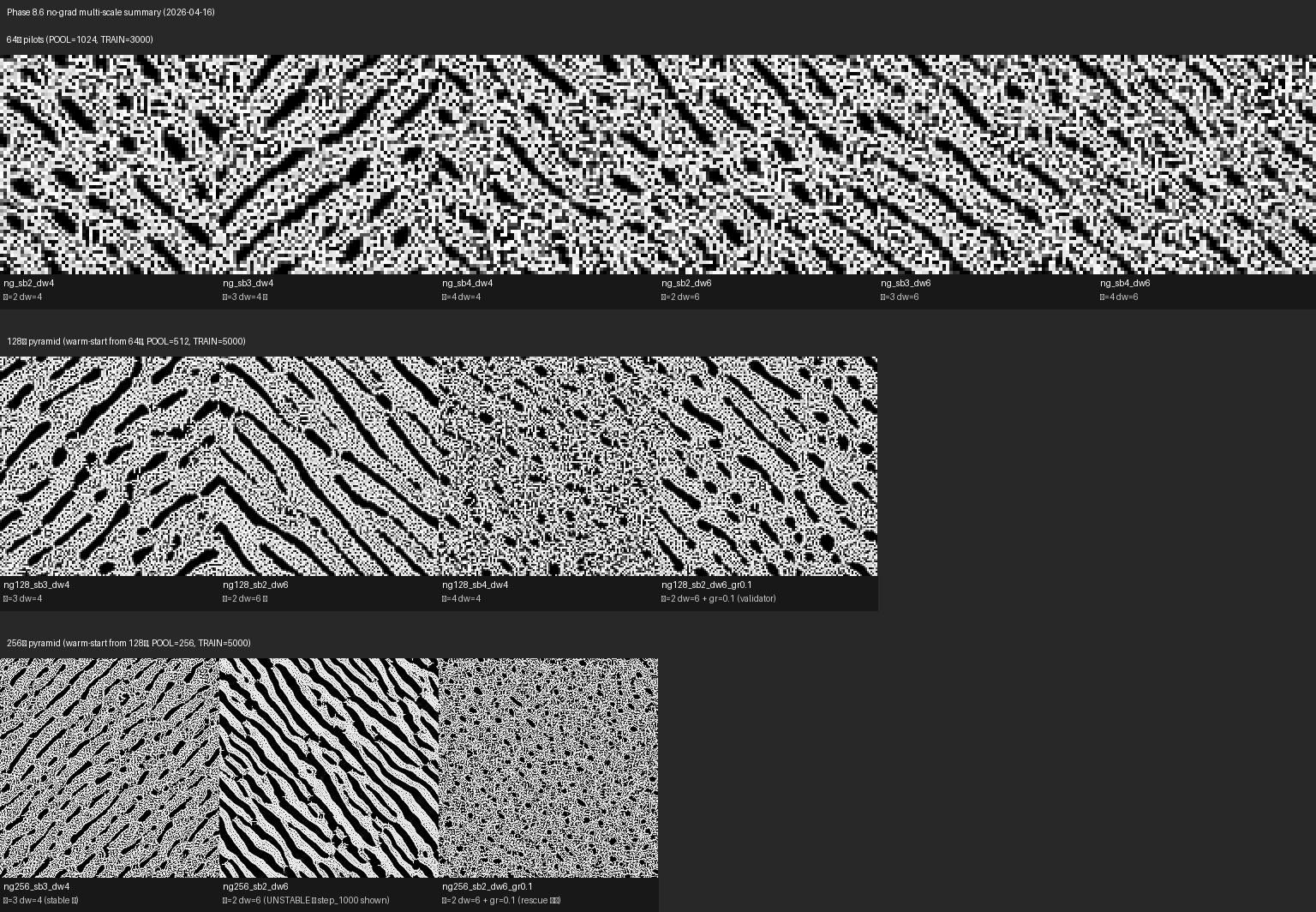
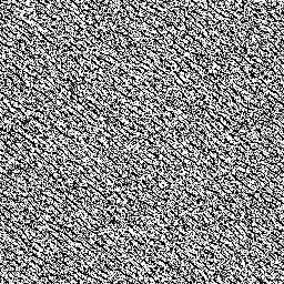
§ 3.04 · phase86_nograd_multiscale·failure family · useful as control
No-gradient multi-scale zoo
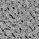
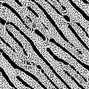
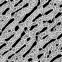
Dropping the Dirichlet gradient term while keeping the multi-scale perception. Without the gradient term, the loss stops being a free-energy minimiser and reduces to a multi-scale heterogeneity maximiser. Whole zoo of attractors emerges, none with the cinematic line-quality of 3.01. Worth keeping for the variety: the σ_blur and double-well-strength axes are the only things the rule can hold onto, and they bend the texture in oddly specific ways.
The frontier of the project as of April 2026. Inject a fBM environment field at every NCA step and ask whether the rule conditions its trajectory on it. Inference-only injection fails; training-time injection works and gives the first conditioned-trajectory evidence.
§ 4.01 · phase86_env_init·negative result
Inference-only injection — the rule erases it
Train without environment, then inject a fractional-Brownian-motion field at inference (R = relu(R + α·fBM) once per step). The hope: the trained kernel uses R as a passive source/sink and the output texture conditions on it.
The kernel erases the injected field within ~45 steps. End state is indistinguishable from training distribution. Heterogeneity has to enter at training time. Stage A is a global attractor.
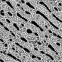
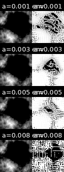
Training under environment — four α, four attractors
Now inject fBM at every NCA step during training. Four warm-started checkpoints diverge as α scales 0.001 → 0.008. The first literal evidence that the same learned rule traces different trajectories under different ambient fields.
§ 4.03 · phase86_env_train_256·frontier · best of phase 8.6
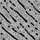
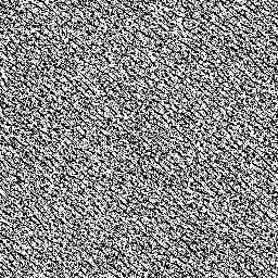
256² beauty shot — vertical wires
Same recipe at 256². α = 0.003 lands on a dense vertical-wire attractor that the 64² runs only hinted at. Same kernel, same training loss, same family. The wider field gives the rule room to lay out finer line structure.
Conservation moved from a soft penalty into the architecture (reintegration tracking transport). Same tension-pair philosophy, different substrate. Result: a translation-invariant spatially-localised pattern. Top 5% of pixels hold 100% of mass; cross-position correlation 0.99+ inside the training distribution.
A clean point in design space, but everything about this attractor is the same shape; there's nothing to vary. Listed here for completeness. Every later card uses soft conservation instead.
a2 · 2ka2 · 5ka2 · 10ka · 5ka · 10kb · 5kb2 · 5k
// 6 · open problems
Pool collapse is the universal terminal failure. Long training collapses the 1024-state pool to similar attractors, gradients homogenise, the rule simplifies. p_reset = 0.01 doesn't supply enough diversity. Higher p_reset or explicit pool-diversity regularisation is the most-likely next lever.
Source/sink ≈ external pool-diversity injection. § 1.04 keeps the "interesting window" open for the whole run, while pure-conservation runs only have a few thousand steps before collapse. Probably the same continuum. The next question is the right kind and strength of external perturbation.
Cardinal four-fold lock in low-T crystal runs (not pictured above; dendrites lock to grid axes under Mullins-Sekerka geometry). Rotation augmentation and hex grids are the next experiments.
Trajectory memory probe. The constraint-geometry argument predicts that learned kernels can encode trajectory information in their state channels. § 4.02 is the first piece of evidence, but no experiment yet distinguishes a state-Markov attractor from a genuinely trajectory-conditioned one.
// 7 · around this — reading list & rabbit-holes
The territory this project sits inside. A casual reading list of things I've read, watched, or kept coming back to. Mix of canonical papers, Wikipedia explainers, author talks, and YouTube popularisations.